Why the Diffusion Module matters in predictive models: a mathematical perspective

In many predictive modeling tasks, the goal is to predict a future or hidden state from observed information. For example:

Predicting future trajectories from historical motion;
Predicting protein structures or functions from sequences;
Predicting future market states from current financial signals;
Predicting disease progression from medical images;
Predicting high-dimensional outputs from contextual information.

A traditional predictive model usually learns a direct mapping:

\[y = f_\theta(x)\]

where $x$ is the input condition, $y$ is the target output, and $f_\theta$ is a neural network parameterized by $\theta$.

This formulation is effective for deterministic prediction problems. However, many real-world predictive tasks are not deterministic. The target is often not a single correct answer, but a conditional probability distribution:

\[p(y \mid x)\]

rather than a single point estimate.

The importance of a diffusion module comes from its ability to model this conditional distribution in a stable, expressive, and mathematically principled way.

1. Prediction is often distribution estimation, not point estimation

Suppose the input is $x$ and the output is $y$. In a standard regression model, we often minimize the mean squared error:

\[\mathcal{L}_{\mathrm{MSE}}(\theta) = \mathbb{E}_{(x,y)} \left[ \left\|y - f_\theta(x)\right\|_2^2 \right]\]

The optimal solution of this objective is the conditional expectation:

\[f_\theta^*(x) = \mathbb{E}[y \mid x]\]

This means that an MSE-trained model tends to predict the average of all possible outcomes.

However, in multimodal prediction problems, the conditional distribution $p(y \mid x)$ may have multiple modes. For the same historical trajectory, a person may turn left, turn right, or go straight. For the same biological sequence, there may be multiple feasible conformations. For the same context, there may be multiple plausible future outputs.

If the model only predicts the conditional mean, it may produce an output that is not realistic.

For example, consider a conditional distribution of the form:

\[p(y \mid x) = 0.5 \mathcal{N}(y; \mu_1, \Sigma_1)+ 0.5 \mathcal{N}(y; \mu_2, \Sigma_2)\]

If $\mu_1$ and $\mu_2$ are far apart, the conditional mean

\[\mathbb{E}[y \mid x] = 0.5\mu_1 + 0.5\mu_2\]

may lie between the two true modes. It may therefore correspond to a low-probability or even invalid outcome.

This is the mathematical reason why many direct prediction models produce blurry, averaged, or low-diversity outputs.

A diffusion module addresses this problem by learning how to generate samples from the full conditional distribution $p(y \mid x)$, rather than predicting only one deterministic output.

2. The core Idea of diffusion: from data to noise, then back

A diffusion model consists of two processes:

A forward diffusion process, which gradually adds noise to real data;
A reverse denoising process, which learns to recover data from noise.

Let the clean target be:

\[y_0 \sim p_{\text{data}}(y)\]

The forward diffusion process is usually defined as:

\[q(y_t \mid y_{t-1}) = \mathcal{N} \left( y_t; \sqrt{1-\beta_t}y_{t-1}, \beta_t I \right)\]

where $\beta_t$ controls the noise level at step $t$, and $T$ denotes the total number of diffusion steps.

After many diffusion steps, $y_T$ becomes approximately standard Gaussian:

\[y_T \sim \mathcal{N}(0, I)\]

In other words, the forward process transforms a complex data distribution into a simple Gaussian distribution.

The reverse process learns:

\[p_\theta(y_{t-1} \mid y_t)\]

which means learning how to move from a noisy sample $y_t$ to a slightly cleaner sample $y_{t-1}$.

After repeated denoising, the model generates a clean sample:

\[y_T \rightarrow y_{T-1} \rightarrow \cdots \rightarrow y_0\]

For prediction tasks, the goal is to model the conditional distribution $p(y \mid x)$, so the reverse process becomes:

\[p_\theta(y_{t-1} \mid y_t, x)\]

That is, the model denoises while being guided by the input condition $x$.

The final output is therefore sampled from:

\[y_0 \sim p_\theta(y \mid x)\]

This is fundamentally different from a deterministic predictor $f_\theta(x)$.

3. Why step-by-step denoising Is easier than direct prediction

A direct predictive model attempts to learn the mapping:

\[x \rightarrow y\]

in one step.

When $p(y \mid x)$ is complex, multimodal, or high-dimensional, this mapping can be highly nonlinear and difficult to approximate.

A diffusion module decomposes the hard problem into many simpler denoising problems:

\[(y_t, x, t) \rightarrow y_{t-1}\]

In practice, the model often predicts the noise added to the clean sample:

\[\epsilon_\theta(y_t, x, t)\]

The noisy sample can be written as:

\[y_t = \sqrt{\bar{\alpha}_t} y_0 + \sqrt{1-\bar{\alpha}_t}\epsilon\]

where:

\[\epsilon \sim \mathcal{N}(0,I)\]

and $\bar{\alpha}_t$ is the cumulative noise schedule coefficient.

The common diffusion training objective is:

\[\mathcal{L}_{\text{diffusion}} = \mathbb{E}*{y_0, x, t, \epsilon} \left[ \left| \epsilon - \epsilon*\theta(y_t, x, t) \right|^2 \right]\]

At first glance, this is simply an MSE loss. But mathematically, it corresponds to learning the score function of the noisy data distribution.

4. The score function: Why diffusion learns distribution geometry

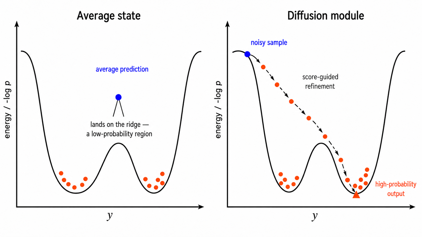
In probabilistic modeling, the score function is defined as:

\[\nabla_y \log p_t(y)\]

It points toward the direction in which the probability density increases most rapidly.

For a conditional noisy distribution $p_t(y_t \mid x)$, if the model can estimate:

\[\nabla_{y_t} \log p_t(y_t \mid x)\]

then it knows how to move a sample from a low-density region toward a high-density region.

In diffusion models, the noise prediction network is closely related to the score function:

\[s_\theta(y_t, x, t) \approx \nabla_{y_t} \log p_t(y_t \mid x)\]

Under a common parameterization:

\[s_\theta(y_t, x, t) = -\frac{1}{\sqrt{1-\bar{\alpha}*t}} \epsilon*\theta(y_t, x, t)\]

Therefore, a diffusion module is not merely learning to remove noise. It is learning the geometry of the target conditional distribution.

In other words, the model learns:

Which regions correspond to realistic outputs;
Which direction a noisy sample should move toward;
Which outputs are likely under condition $x$;
How to transform random noise into high-probability predictions.

From this perspective, a diffusion module acts as an implicit conditional distribution gradient estimator.

5. Role 1: Modeling multimodal uncertainty

Uncertainty in predictive modeling can be divided into two major types.

5.1 Aleatoric uncertainty

Aleatoric uncertainty is the inherent randomness in the data-generating process. For example, under the same condition $x$, there may be several valid future outcomes.

Mathematically, this means that:

\[p(y \mid x)\]

is not a sharp single-mode distribution, but a broad or multimodal distribution.

5.2 Epistemic uncertainty

Epistemic uncertainty comes from limited data, model uncertainty, or insufficient generalization.

A traditional point predictor only produces:

\[\hat{y} = f_\theta(x)\]

Even if the model predicts a variance, it often assumes a simple Gaussian distribution:

\[p(y \mid x) = \mathcal{N} \left( \mu_\theta(x), \sigma_\theta^2(x)I \right)\]

This assumption is often too restrictive for complex real-world prediction tasks.

A diffusion module can naturally produce multiple plausible predictions by sampling:

\[y^{(1)}, y^{(2)}, \ldots, y^{(K)} \sim p_\theta(y \mid x)\]

This allows the model to answer not only “What is the most likely outcome?”, but also:

What other outcomes are plausible?
How diverse are the possible predictions?
Which modes are stable?
Where is the predictive uncertainty high?

This makes diffusion especially valuable in probabilistic prediction, diversity-aware forecasting, and risk-sensitive decision making.

6. Role 2: Improving expressiveness in high-dimensional output spaces

In many modern prediction problems, the output $y$ is not a low-dimensional scalar. It may be a high-dimensional structured object:

Image prediction: $y \in \mathbb{R}^{H \times W \times C}$
Molecular conformation prediction: $y \in \mathbb{R}^{N \times 3}$
Trajectory prediction: $y \in \mathbb{R}^{T \times d}$
Sequence prediction: $y \in \mathbb{R}^{L \times V}$
Gene expression prediction: $y \in \mathbb{R}^{G}$

In high-dimensional spaces, real data often lie near a low-dimensional manifold:

\[y \in \mathcal{M} \subset \mathbb{R}^D\]

A direct regression model may produce outputs that are close to the target under MSE, but still far from the true data manifold. Such predictions may be numerically reasonable but physically, biologically, or semantically invalid.

The denoising process in a diffusion model can be interpreted as gradually moving samples back toward the data manifold:

\[y_T \rightarrow y_{T-1} \rightarrow \cdots \rightarrow y_0 \in \mathcal{M}\]

Each denoising step uses the estimated score function to push samples toward high-density regions.

Thus, in high-dimensional prediction tasks, a diffusion module acts as a structured prior:

\[p_\theta(y \mid x)\]

It helps constrain predictions to lie near realistic regions of the output space.

7. Role 3: Turning prediction into conditional generation

A traditional prediction model is usually written as:

\[\hat{y} = f_\theta(x)\]

A diffusion-based prediction model instead starts from noise:

\[y_T \sim \mathcal{N}(0,I)\]

and iteratively applies conditional denoising:

\[y_{t-1} = g_\theta(y_t, x, t) + \sigma_t z\]

where:

\[z \sim \mathcal{N}(0,I)\]

The final prediction is:

\[\hat{y} = y_0\]

The key difference is that prediction is no longer a deterministic function. It becomes a stochastic generative process.

The full conditional distribution can be written as:

\[p_\theta(y \mid x) = \int p(y_T) \prod_{t=1}^{T} p_\theta(y_{t-1} \mid y_t, x) dy_{1:T}\]

This equation is central. It shows that the diffusion module constructs a complex conditional distribution through a sequence of simpler conditional transition distributions.

Each individual transition may be relatively simple, but their composition can represent highly complex distributions.

This is analogous to decomposing a complex mapping into a composition of many small transformations:

\[F = f_1 \circ f_2 \circ \cdots \circ f_T\]

From an expressiveness perspective, this multi-step formulation is more flexible than one-step prediction.

8. Role 4: Stable training objective

There are many generative modeling frameworks, including GANs, VAEs, normalizing flows, and autoregressive models. A major advantage of diffusion models is their relatively stable training objective.

The core training objective is usually noise regression:

\[\mathcal{L} = \mathbb{E} \left[ |\epsilon - \epsilon_\theta(y_t, x, t)|^2 \right]\]

Compared with the minimax objective of GANs:

\[\min_G \max_D \mathbb{E}*{y \sim p*{\text{data}}} [\log D(y)] + \mathbb{E}_{z \sim p_z} [\log(1-D(G(z)))]\]

diffusion models do not require a discriminator and are less prone to mode collapse.

For predictive models, this matters because prediction systems often require:

Stable outputs;
Coverage of multiple possible mode;
Preservation of rare but important outcomes;
Smooth behavior under small changes in the input condition.

Since the diffusion objective is a supervised noise-prediction loss, it is often easier to integrate into existing predictive architectures.

9. Role 5: Controllability and conditional constraints

In prediction tasks, we do not want to generate arbitrary samples. We want outputs that are strongly conditioned on $x$.

Conditional diffusion uses the reverse process:

\[p_\theta(y_{t-1} \mid y_t, x)\]

Here, $x$ may represent:

Text conditions;
Historical time series;
Graph structures;
Biological sequences;
Physical parameters;
Experimental conditions;
Multimodal context.

Guidance methods can further adjust the strength of conditioning. For example, classifier-free guidance is commonly written as:

\[\epsilon_{\mathrm{guided}} = \epsilon_\theta(y_t,\varnothing,t) + w\Bigl[ \epsilon_\theta(y_t,x,t) - \epsilon_\theta(y_t,\varnothing,t) \Bigr].\]

where $w$ is the guidance scale.

When $w$ increases, the model tends to generate outputs that conform more strongly to condition $x$. When $w$ decreases, the outputs usually preserve more diversity.

This gives predictive models a useful control mechanism:

Stronger conditioning for conservative prediction;
Weaker conditioning for diverse candidate generation;
Modified sampling strategies for rare-event exploration;
Constraint-guided denoising for physical or biological validity.

Thus, a diffusion module does not merely produce predictions. It provides a controllable prediction mechanism.

10. A bayesian view of diffusion-based prediction

From a Bayesian perspective, prediction can be written as:

\[p(y \mid x) = \frac{p(x \mid y)p(y)}{p(x)}\]

where:

$p(y)$ is the prior over the output space;
$p(x \mid y)$ is the observation model;
$p(y \mid x)$ is the posterior predictive distribution.

Many traditional models directly approximate $p(y \mid x)$ without explicitly learning a rich prior over $y$.

A diffusion module can be interpreted as learning a powerful data prior:

\[p_\theta(y)\]

or, in conditional prediction:

\[p_\theta(y \mid x)\]

This prior helps the model rule out unrealistic outputs and encourages predictions that respect the structure of the data.

This is especially important in high-dimensional spaces, where most possible points are meaningless. The model must know which regions correspond to valid samples, and the diffusion denoising process provides this probabilistic constraint.

11. A simple example: diffusion for trajectory prediction

Suppose we want to predict a future trajectory $y$ from a historical trajectory $x$.

For the same historical trajectory, there may be three possible future modes:

\[p(y \mid x) = \pi_1 p_1(y \mid x) + \pi_2 p_2(y \mid x) + \pi_3 p_3(y \mid x)\]

These modes may correspond to:

Turning left;
Turning right;
Going straight.

If we use MSE regression, the model may predict the average trajectory:

\[\hat{y} = \pi_1 \mu_1 + \pi_2 \mu_2 + \pi_3 \mu_3\]

This average trajectory may not correspond to any realistic future.

In contrast, a diffusion-based predictor can sample multiple initial noises:

\[y_T^{(k)} \sim \mathcal{N}(0,I)\]

and generate multiple plausible futures:

\[y_0^{(k)} \sim p_\theta(y \mid x)\]

As a result, the model can generate left-turn, right-turn, and straight trajectories simultaneously, rather than collapsing them into a single averaged prediction.

This is one of the clearest reasons why diffusion modules are valuable in predictive modeling.

12. Mathematical comparison with traditional prediction modules

Method	Learning Target	Output Form	Distribution Expressiveness	Multimodal Prediction
MSE Regression	$\mathbb{E}[y \mid x]$	Single point	Weak	Weak
Gaussian NLL	$\mu(x), \sigma(x)$	Single Gaussian	Moderate	Limited
Mixture Density Network	Mixture parameters	Explicit mixture distribution	Strong	Strong
VAE	Latent-variable generation	Random samples	Strong	Strong
GAN	Adversarial generation	Random samples	Strong	May suffer from mode collapse
Diffusion	Conditional denoising process	Multi-step samples	Very strong	Strong

The point is not that diffusion is always superior. Rather, diffusion modules are especially attractive when:

The output space is high-dimensional;
The target distribution is multimodal;
Multiple candidate predictions are needed;
Both sample quality and distribution coverage matter;
Stable training is important;
Conditional control or constraint guidance is required.

13. Why diffusion modules integrate naturally with deep predictive models

Modern predictive systems usually already have a powerful encoder:

\[h = \text{Encoder}_\phi(x)\]

where $h$ is the latent representation of the input condition.

A diffusion module can then serve as a probabilistic decoder:

\[\epsilon_\theta(y_t, h, t)\]

The full predictive architecture becomes:

\[h = \text{Encoder}_\phi(x)\] \[y_0 \sim \text{DiffusionDecoder}_\theta(h)\]

This structure is natural:

The encoder understands the condition;
The diffusion decoder models the complex output distribution;
The denoising process generates high-quality samples consistent with the condition.

Therefore, diffusion modules can be incorporated into many existing predictive architectures, such as:

Transformer encoder + diffusion decoder;
GNN encoder + diffusion decoder;
CNN encoder + diffusion decoder;
Protein language model + diffusion structure decoder;
Time-series encoder + diffusion trajectory decoder.

From a modular design perspective, a diffusion module is a powerful probabilistic decoder.

14. Limitations of diffusion modules…

Although diffusion modules are powerful, they also have costs.

14.1 Slow sampling

The generation process requires multiple denoising steps:

\[T, T-1, \ldots, 1\]

If $T$ is large, inference can be computationally expensive.

14.2 Sensitivity to noise scheduling

The noise schedule $\beta_t$ affects both training and sampling quality. Different tasks may require different schedules.

14.3 More complex evaluation

Point predictors can be evaluated with MSE, MAE, or related metrics. Diffusion-based predictors output distributions, so evaluation may require additional metrics:

Likelihood;
Calibration;
Coverage;
Diversity;
Sample quality;
Downstream utility.

14.4 Not always necessary

If the task is nearly deterministic or the output dimension is low, a simple regression model may be sufficient. The advantages of diffusion modules are most significant in complex, high-dimensional, and multimodal prediction problems.

15. Conclusion

Mathematically, the importance of a diffusion module in predictive models can be summarized as follows.

First, prediction often requires learning a conditional distribution:

\[p(y \mid x)\]

rather than a deterministic mapping:

\[y = f_\theta(x)\]

Second, diffusion models represent a complex conditional distribution through a sequence of simple denoising transitions:

\[p_\theta(y \mid x) = \int p(y_T) \prod_{t=1}^{T} p_\theta(y_{t-1} \mid y_t, x) dy_{1:T}\]

Third, the noise prediction objective is closely related to learning the score function of the data distribution:

\[\nabla_y \log p_t(y \mid x)\]

This gives the model information about how to move samples toward high-probability regions.

Fourth, diffusion modules naturally model multimodal uncertainty and avoid the averaging effect of MSE regression.

Fifth, in high-dimensional output spaces, diffusion modules provide a powerful data-manifold prior that encourages predictions to be realistic, structured, and conditionally valid.

Therefore, a diffusion module is not merely a generative component. It is a probabilistic modeling mechanism. It transforms prediction from “producing one answer” into “characterizing the distribution of all plausible answers.”

For complex system prediction, this shift is often what determines the upper bound of model capability.

References

Foundational diffusion models

Ho, J., Jain, A., & Abbeel, P. (2020). Denoising Diffusion Probabilistic Models. Advances in Neural Information Processing Systems 33.
Song, J., Meng, C., & Ermon, S. (2020). Denoising Diffusion Implicit Models.
Song, Y., Sohl-Dickstein, J., Kingma, D. P., Kumar, A., Ermon, S., & Poole, B. (2021). Score-Based Generative Modeling through Stochastic Differential Equations. International Conference on Learning Representations.
Ho, J., & Salimans, T. (2022). Classifier-Free Diffusion Guidance.

Recent AI4Science papers

Abramson, J., Adler, J., Dunger, J., et al. (2024). Accurate structure prediction of biomolecular interactions with AlphaFold 3. Nature.
Protenix Team. (2025). Protenix: Advancing Structure Prediction Through a Comprehensive AlphaFold3 Reproduction. bioRxiv.
Xu, M., et al. (2025). Efficient protein structure generation with sparse denoising models. Nature Machine Intelligence.
Wang, et al. (2026). Two-dimensional geometric template diffusion for boosting single-sequence protein structure prediction. Nature Machine Intelligence.
Cheng, K., Liu, C., Su, Q., Wang, J., Zhang, L., Tang, Y., Yao, Y., Zhu, S., & Qi, Y. (2024). 4D Diffusion for Dynamic Protein Structure Prediction with Reference Guided Motion Alignment. arXiv.
Liu, et al. (2026). DCFold: Efficient Protein Structure Generation with Single-step Diffusion. arXiv.
Qiang, B., Gong, C., Chen, X., Zhang, Y., & Xiao, W. (2025). Protenix-Mini+: efficient structure prediction model with scalable pairformer. arXiv.
Yi, Z., Chan, L., Yiming, M., Wei, Q., Fei, Y., Kexin, Z., Lan, W., Minrui, G., & Quanquan, G. (2025). SeedFold: Scaling Biomolecular Structure Prediction. arXiv.